Finite Difference Analysis (FDA) and cosine_similarity
Foreword
Nothing fancy here — I just felt like writing something.
In a Nishika competition, yama brought up the Negative Cosine Similarity Loss and wired it up as a custom loss for lgbm.
→ yama’s notebook
This article is also posted on Qiita.
The finite difference trick and how it gets applied there struck me as genuinely interesting, so I wanted to make it the subject of my first blog post.
I won’t get into how well the loss actually performs in that competition. What I want to talk about is how an lgbm loss function works and how finite differences come into play.
Finite Difference Analysis
Finite Difference Analysis is one of the workhorse techniques in numerical analysis and mathematical modeling. You use it to approximate the derivative of a function or an equation.
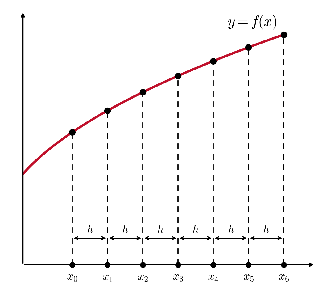
It comes in three flavors: forward difference, central difference, and backward difference.
1. Forward Difference
To approximate the derivative of $f(x)$ at a point $x$, the forward difference uses the function value at a point slightly ahead, $x+h$, and subtracts the value at $x$. The formula is:
$$ f’(x) \approx \frac{f(x + h) - f(x)}{h} $$
where $h$ is a very small number. In other words, it measures the rate of change looking forward from $x$.
2. Central Difference
To approximate the derivative of $f(x)$ at $x$, the central difference uses the values at the points on either side, $x+h$ and $x-h$. The formula is:
$$ f’(x) \approx \frac{f(x + h) - f(x - h)}{2h} $$
The central difference gives a more accurate estimate of the rate of change at $x$, and in general it’s more precise than the forward difference.
3. Backward Difference
To approximate the derivative of $f(x)$ at $x$, the backward difference uses the value at a point slightly behind, $x-h$, and subtracts it from the value at $x$. The formula is:
$$ f’(x) \approx \frac{f(x) - f(x - h)}{h} $$
This measures the rate of change looking backward from $x$.
4. What’s the difference?
All three rely on points near where the function is evaluated. The only real distinction is whether you look forward or backward — and which one matters is dictated by the function itself: is the information ahead of the point more important, or the information behind it?
That said, the central difference is generally regarded as the most accurate of the three.
5. A concrete example
Say we want the derivative of $f(x)=x^2$ at $x = 4$. With the central difference:
$$ f’(4) \approx \frac{f(4 + h) - f(4 - h)}{2h} $$
You then shrink $h$ and compute.
A simple application, and deriving the formulas
—— How do we get the first and second derivatives of a function using finite differences?
1. First derivative — the gradient
The first derivative is the slope of the function.
Suppose we want the first derivative of $f(x)$ at the point $x_0$. From the Taylor expansion, we can write the value of $f(x)$ near $x_0$ as:
$$ f(x) = f(x_0) + f’(x_0)(x-x_0) + \frac{f’’(x_0)}{2!}(x-x_0)^2 + \cdots $$
Everything after this is a higher-order infinitesimal, so keeping only the first two terms gives:
$$ f(x) \approx f(x_0) + f’(x_0)(x-x_0) $$
Setting $x$ to $x_0 + dx$ and $x_0 - dx$:
$$ f(x_0 + dx) \approx f(x_0) + f’(x_0)dx $$
$$ f(x_0 - dx) \approx f(x_0) - f’(x_0)dx $$
Subtracting the second from the first:
$$ f(x_0 + dx) - f(x_0 - dx) \approx 2f’(x_0)dx $$
which gives us the finite difference formula:
$$ f’(x_0) \approx \frac{f(x_0 + dx) - f(x_0 - dx)}{2dx} $$
2. Second derivative — the Hessian matrix
The second derivative is the rate of change of the first derivative — also called the curvature. It’s the derivative of the derivative, i.e. the gradient of the gradient, and that’s what the Hessian matrix captures.
The second derivative works the same way, except now the Taylor expansion keeps the first three terms:
$$ f(x) \approx f(x_0) + f’(x_0)(x-x_0) + \frac{f’’(x_0)}{2!}(x-x_0)^2 $$
Setting $x$ to $x_0 + dx$ and $x_0 - dx$:
$$ f(x_0 + dx) \approx f(x_0) + f’(x_0)dx + \frac{f’’(x_0)}{2!}dx^2 $$
$$ f(x_0 - dx) \approx f(x_0) - f’(x_0)dx + \frac{f’’(x_0)}{2!}dx^2 $$
Adding the two:
$$ f(x_0 + dx) + f(x_0 - dx) \approx 2f(x_0) + f’’(x_0)dx^2 $$
which gives the finite difference formula:
$$ f’’(x_0) \approx \frac{f(x_0 + dx) + f(x_0 - dx) - 2f(x_0)}{dx^2} $$
3. cosine_similarity as the example
Let’s take the cosine_similarity from yama’s code as our example.
Given two vectors, pred and true, cosine similarity measures how alike they are:
$$ \text{Cosine Similarity}(\mathbf{pred}, \mathbf{true}) = \frac{\mathbf{pred} \cdot \mathbf{true}}{|\mathbf{pred}| |\mathbf{true}|} $$
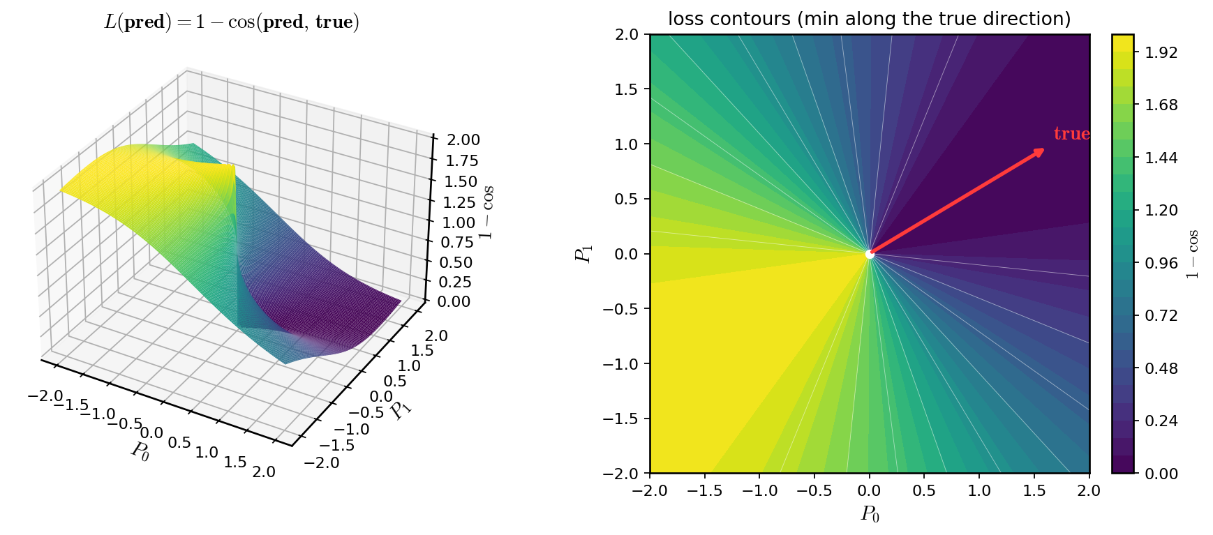
Treating $1 - \cos$ as the loss and holding true fixed, the landscape looks like this — the loss bottoms out wherever pred points in the same direction as true.

First derivative / gradient
For $f(pred, true)$, computing with the central difference gives:
$$ \nabla f(\mathbf{pred}, \mathbf{true}) \approx \frac{f(\mathbf{pred} + \Delta\mathbf{pred}, \mathbf{true} + \Delta\mathbf{true}) - f(\mathbf{pred} - \Delta\mathbf{pred}, \mathbf{true} - \Delta\mathbf{true})}{2\epsilon} $$
where $\Delta\mathbf{pred}$ and $\Delta\mathbf{true}$ are small vector increments and $\epsilon$ is a small positive number.
Second derivative / Hessian matrix
$$ \nabla^2 f(\mathbf{pred}, \mathbf{true}) \approx \frac{\nabla f(\mathbf{pred} + \Delta\mathbf{pred}, \mathbf{true} + \Delta\mathbf{true}) - \nabla f(\mathbf{pred} - \Delta\mathbf{pred}, \mathbf{true} - \Delta\mathbf{true})}{2\epsilon} $$
To put it more plainly:
When you differentiate or take differences of a vector, you do it for each element separately — one partial derivative or difference at a time.
That’s because each element of the vector is assumed to be independent of the others.
For a 2D vector $pred = [P_0,P_1]$, for instance, the first-order partials (the gradient) of cosine_similarity are:
$$ \frac{\partial f}{\partial P_0} \approx \frac{f([P_0 + \Delta P_0, P_1], \mathbf{true}) - f([P_0 - \Delta P_0, P_1], \mathbf{true})}{2\epsilon} $$
$$ \frac{\partial f}{\partial P_1} \approx \frac{f([P_0, P_1 + \Delta P_1], \mathbf{true}) - f([P_0, P_1 - \Delta P_1], \mathbf{true})}{2\epsilon} $$
So the gradient is:
$$ \nabla f(\mathbf{pred},\mathbf{true}) = \left[\frac{\partial f}{\partial P_0}, \frac{\partial f}{\partial P_1}\right] $$
And the Hessian follows the same way:
$$ \frac{\partial^2 f}{\partial P_0^2} \approx \frac{f([P_0 + 2\Delta P_0, P_1], \mathbf{true}) - 2f([P_0 + \Delta P_0, P_1], \mathbf{true}) + f([P_0, P_1], \mathbf{true})}{\epsilon^2} $$
$$ \frac{\partial^2 f}{\partial P_1^2} \approx \frac{f([P_0, P_1 + 2\Delta P_1], \mathbf{true}) - 2f([P_0, P_1 + \Delta P_1], \mathbf{true}) + f([P_0, P_1], \mathbf{true})}{\epsilon^2} $$
$$ \frac{\partial^2 f}{\partial P_0 \partial P_1} = \frac{\partial^2 f}{\partial P_1 \partial P_0} \approx \frac{f([P_0 + \Delta P_0, P_1 + \Delta P_1], \mathbf{true}) - f([P_0 + \Delta P_0, P_1 - \Delta P_1], \mathbf{true})}{4\epsilon^2} $$
$$ \nabla^2 f(\mathbf{pred}, \mathbf{true}) = \left[\frac{\partial^2 f}{\partial P_0^2}, \frac{\partial^2 f}{\partial P_1^2}, \frac{\partial^2 f}{\partial P_0 \partial P_1}\right] $$
Python
I’m quoting yama’s code directly.
I made a couple of small tweaks, which I’ll explain at the end.
def derivative(y_pred, y_true, dx):
    n = y_pred.shape[0]
    grad = np.zeros(n)
    hess = np.zeros(n)
    z_true = np.sqrt((y_true ** 2).sum())
    f_0 = 1 -1 * (y_pred * y_true).sum() / np.sqrt((y_pred ** 2).sum()) / z_true
    for i in range(n):
        y_pred[i] = y_pred[i] - dx
        f_m = 1 -1 * (y_pred * y_true).sum() / np.sqrt((y_pred ** 2).sum()) / z_true
        y_pred[i] = y_pred[i] + dx + dx
        f_p = 1 -1 * (y_pred * y_true).sum() / np.sqrt((y_pred ** 2).sum()) / z_true
        y_pred[i] = y_pred[i] - dx
        grad[i] = (f_p - f_m) / (dx * 2)
        hess[i] = (f_p + f_m - 2 * f_0) / (dx ** 2)

    return grad, hess

# Negative cosine similarity
# Pass this as the LightGBM objective.
def negative_cosine_similarity_loss(y_pred, data):
    y_true = np.double(data.get_label())
    grad, hess = derivative(y_pred, y_true, 1e-3)

    return grad, hess
Here, f0 is the value at the original point:
$$ f_0 = 1 - \frac{\sum{(y_{pred} \cdot y_{true})}}{|y_{pred}| \cdot |y_{true}|} $$
That is, $(1 - cosine\ similarity)$. Subtracting from 1 maps the range from $[-1,1]$ to $[2,0]$; after the transform it becomes the angular loss.
The upside is generality — whatever you do to drive the loss value down carries over. The downside is that the loss values you see during experiments aren’t as intuitive to read.
Whether to remap the range is a call you make depending on the situation.
$fm\ (f_{minus})$: the function value after subtracting a small positive $dx$ from $y_{pred}[i]$. It can be written as:
$$ fm = f(y_{pred} - [0, …, 0, dx, 0, …, 0], y_{true}) $$
$fp\ (f_{plus})$: the function value after adding a small positive $dx$ to $y_{pred}[i]$:
$$ fp = f(y_{pred} + [0, …, 0, dx, 0, …, 0], y_{true}) $$
In short, you loop over the predictions and apply the finite difference once to each, building up grad and hess — the gradient and the Hessian.
At which point you may have noticed: the Hessian here is missing the third component mentioned earlier. There’s no mixed partial $\frac{\partial^2 f}{\partial P_0 \partial P_1}$.
That’s because LightGBM isn’t a Newton-style optimizer — it uses Gradient Boosting Trees as its base learner.
lgbm builds the model primarily from gradient information, without ever computing or using the third component of the Hessian. So you only need the first derivative (the gradient) and the second derivative restricted to the diagonal of the Hessian (e.g. $[\frac{\partial^2 f}{\partial P_0^2}, \frac{\partial^2 f}{\partial P_1^2}]$).
These are what drive the split rules and the leaf-value updates that construct the tree model, with no need to consider the off-diagonal terms of the Hessian. The result is lower compute cost and more efficient training.