IceCube - Neutrinos in Deep Ice

Foreword

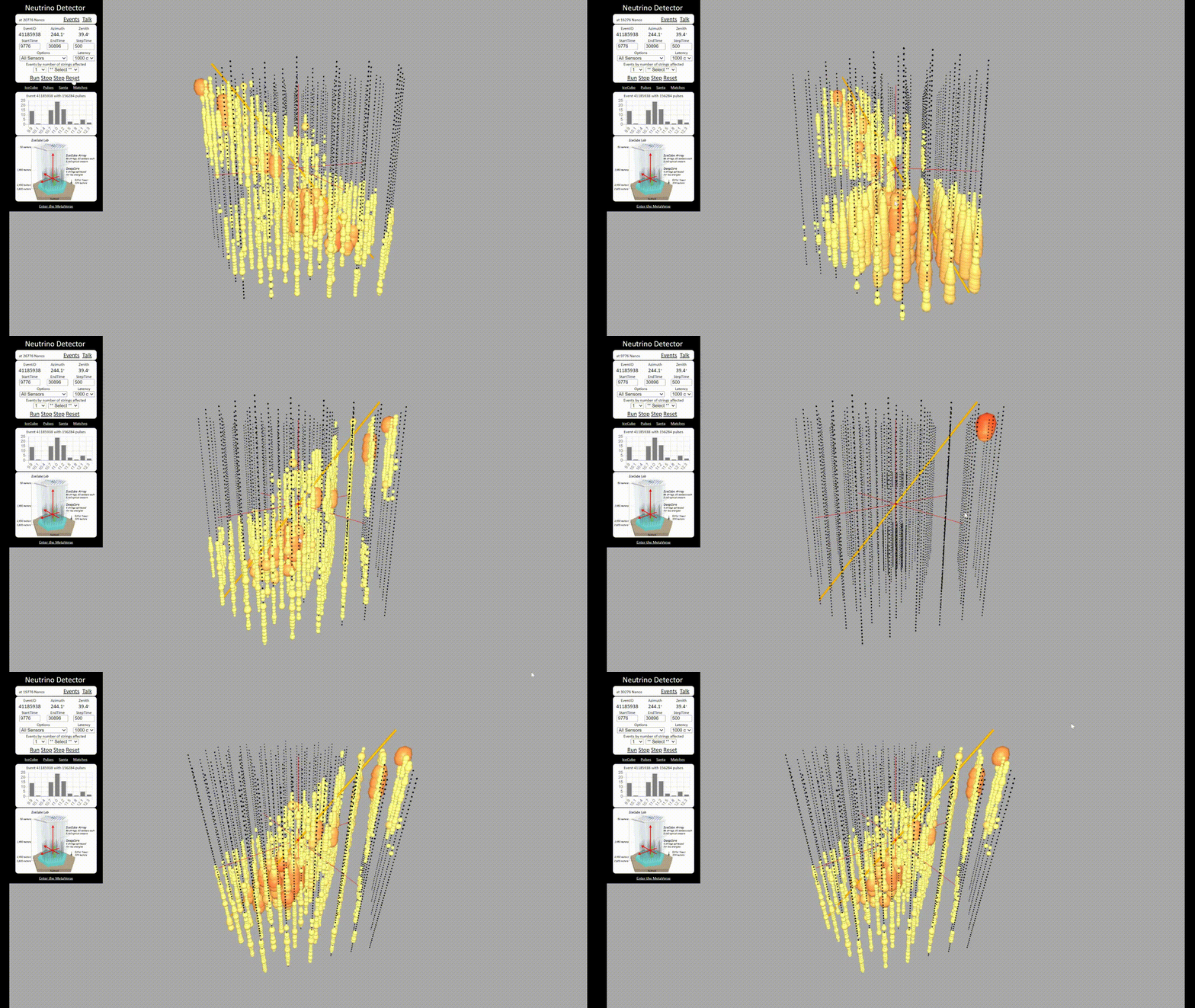
I am writing this article in the hope of sharing insights from my personal journey in the competition, accompanied by a brief introduction to the techniques employed.

After completing the IceCube Kaggle challenge, I decided to summarize my insights in innovation points and methods I learned on the way.

For a detailed explanation, I highly recommend delving into the outstanding paper authored by Habib Bukhari, Dipam Chakraborty, Philipp Eller, et al.[8].

Introduction

One of the most abundant particles in the universe is the neutrino. While similar to an electron, the nearly massless and electrically neutral neutrinos have fundamental properties that make them difficult to detect. Yet, to gather enough information to probe the most violent astrophysical sources, scientists must estimate the direction of neutrino events. If algorithms could be made considerably faster and more accurate, it would allow for more neutrino events to be analyzed, possibly even in real-time and dramatically increase the chance to identify cosmic neutrino sources. Rapid detection could enable networks of telescopes worldwide to search for more transient phenomena.

Researchers have developed multiple approaches over the past ten years to reconstruct neutrino events. However, problems arise as existing solutions are far from perfect. They’re either fast but inaccurate or more accurate at the price of huge computational costs.

The IceCube Neutrino Observatory is the first detector of its kind, encompassing a cubic kilometer of ice and designed to search for the nearly massless neutrinos. An international group of scientists is responsible for the scientific research that makes up the IceCube Collaboration. [1]

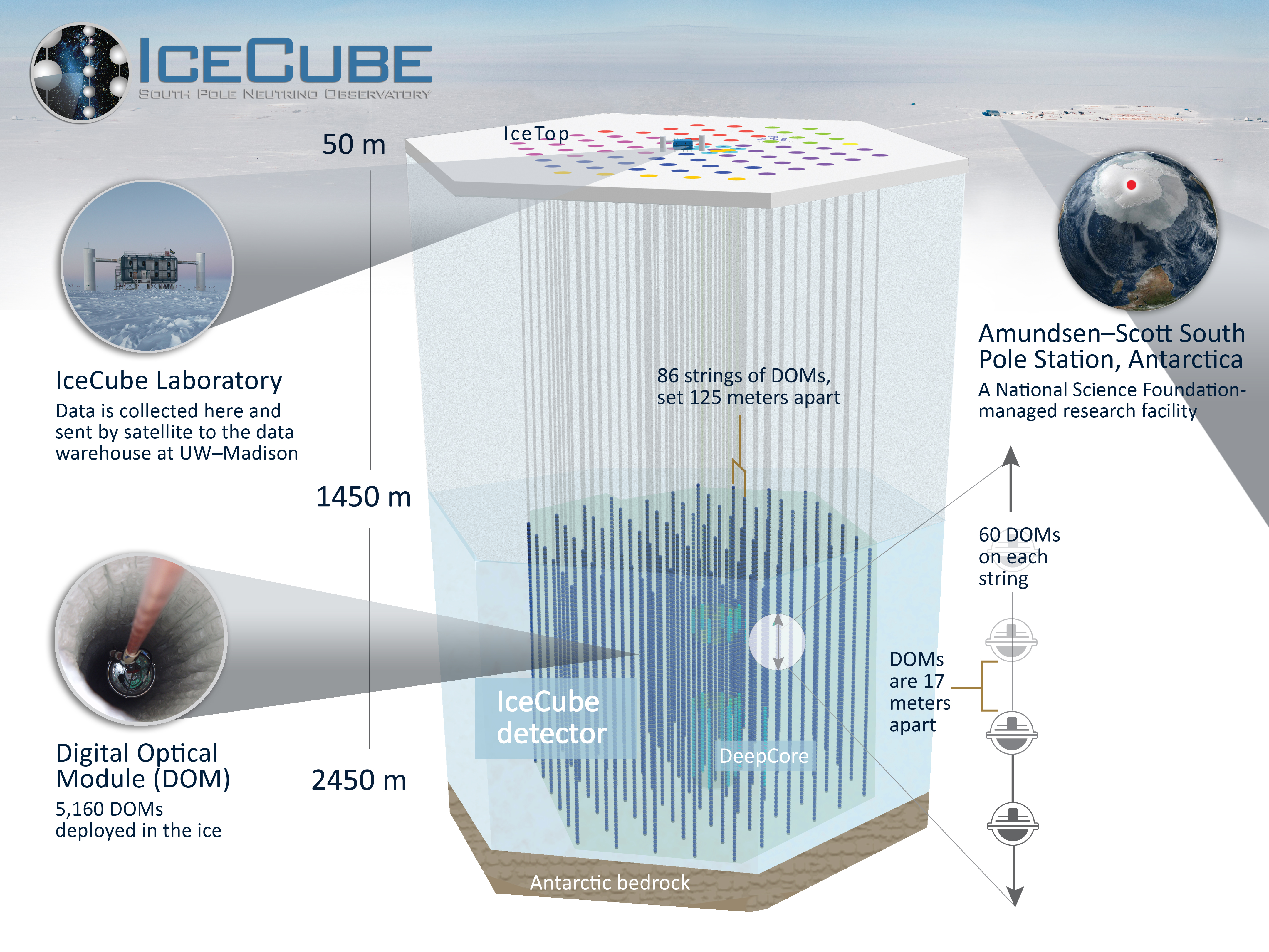
Figure1 IceCube

Icecube detects neutrinos primarily by detecting the Cherenkov light. Cherenkov light is an electromagnetic radiation emitted when charged particles pass through a dielectric at a speed greater than the phase velocity of light in the medium (the speed at which the wavefront travels through the medium). Simple analogy to it is the sonic wave from explosion but Cherenkov light is a shock wave of light. So when neutrinos and nuclei react they produce charged secondary particles, which in turn produce Cherenkov light. Then IceCube’s Digital Optical module (DOM) detects this light after a neutrino passed through.

Therefore, in the competition, we use the energy of pulsing light, the duration of the detection, and sensor coordinates to indirectly predict the neutrino’s path defined by zenith and azimuth angles.

Challenges

Detecting low-energy particles has always been a scientific problem for decades. Therefore, there are few possible difficulties arising from 2 following factors:

1. Detector sensitivity. Icecube is designed to observe neutrinos with energies of about one-tenth of a TeV. Although the DeepCore subdetector extends this range to 50 GeV, allowing the detection of low-energy neutrinos, there are still neutrinos with even lower energy.
2. Noise from other particles. Muons, produced by the interaction of cosmic rays with the Earth’s atmosphere, can outnumber neutrino signals in IceCube. Approximately 1,000,000 muons are detected for every neutrino seen in IceCube.[5]

The Least Square

Least squares is a simple statistical approach, that was utilised for problem analysis [2,3,4]. The core idea of this method is that if the pulse light is propagated in an omni-directional manner due to a neutrino collision, the time-weighted omni-directional properties should cancel each other out, leaving only the properties of the neutrino’s path.

Thus, if we replace the charge with the mass we will obtain the “center of charge”, which is equivalent to the center of mass. This allows us to get two points, apply least squares regression and draw a line from the earliest point to the latest point.

Let $𝒗_𝒊$ be the x,y, and z coordinates of the observed value, and $𝒕𝟎_𝒊 (𝒕𝟏_𝒊)$ be the time weight, then we can simply get:

$$ v_0 = \frac{\sum(v_i \cdot charge_i \cdot t0_i)}{\sum(charge_i \cdot t0_i)} $$ $$ v_1 = \frac{\sum(v_i \cdot charge_i \cdot t1_i)}{\sum(charge_i \cdot t1_i)} $$

then $v_1-v_0$ is the direction vector of the neutrino, and its opposite is the direction of the source of the neutrino, that is, the value to be predicted.

Because of these properties, least squares regression is a suitable method for approximation of neutrino’s trajectory. However, there are still many problems with this approach. The points used to perform the algorithm may not be strictly symmetric, and there may be pulse events that happen below sensitivity range of the detector. Due to the development of statistical methods, this approach currently falls behind other methods, but is very important for understanding of the problem.

DynEdge

We decided to approach the problem using Graph Neural Networks (GNN), specifically employing DynEdge from Graphnet for the task of neutrino reconstruction and classification.

Experimental results from the original paper demonstrate that DynEdge excels in performance, particularly for low-energy neutrinos, outperforming other contemporary methods. Consequently, DynEdge became the focal point of our efforts in this stage.

A main technology in this model is the EdgeConv operator, crucial for convolution on point cloud images and identified by researchers themselves as the one suitable for the analysis of data from detector [11]. The main structure of EdgeConv is illustrated in Figure 2.

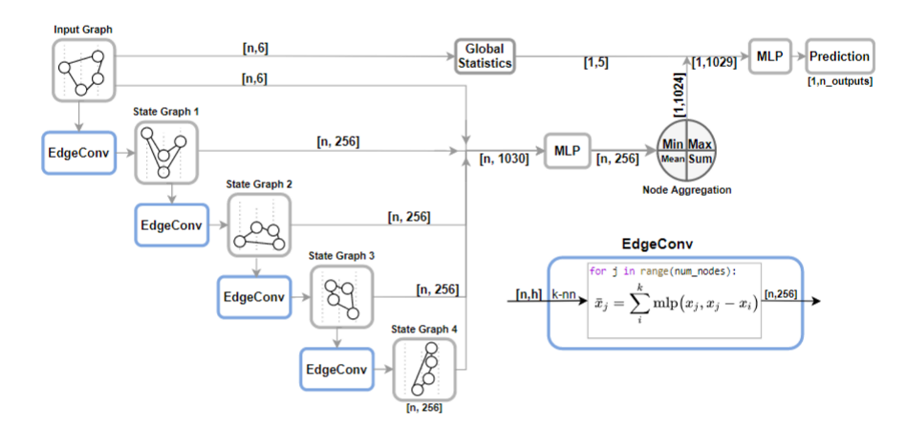
Figure2 Structure of Graphnet

The mathematical representation indicates that for each node 𝑛 𝑗 with node features 𝑥 𝑗 , the operator convolves 𝑥 𝑗 within the local neighborhood of 𝑛 𝑗 as:

$$ x_j = \sum_{i=1}^{N_{neighbors}} MLP(x_j - x_i) $$

Here, $x_j$ represents the convolved node features of $n_j$, and the Multilayer Perceptron (MLP) takes as input the unconvolved node features of $n_j$ and the pairwise difference between the unconvolved node features of $n_j$ and its $i$-th neighbor. [4, 8]

In essence, EdgeConv receives node features and their differences from neighbors, convolving them on the graph. Notably, its “convolution kernel” is determined by the number of links, meaning the “kernel” is defined by the edge, not its location. As depicted in the lower right corner of Figure 2, this step allows DynEdge to link arbitrary nodes in each convolution step, providing enhanced flexibility and a more comprehensive inclusion of intrinsic features between points, beyond just their coordinates.

The score improved, but my position in ranking is still middling.

Switch to RNN

In the third stage, I, and most of the kagglers, switched to RNN.

In retrospect, this seems like a very natural idea, it seems logical that neutrinos would pass through the detector over period of time.

Transform regression task into classification task

The idea comes from the paper [6].

This is an important step in the LSTM solution. The approach involves partitioningzenith and azimuth angles into 24 segments each, encoding them using base 24, and transform the regression task into a classification task. Following this, the predicted values seamlessly map back to the regions encoded with 24.

This method greatly improved the score.

Different structures and ensembles

There’s not a lot to explain. I simply designed a variety of LSTM and GRU combination structures, and weighted them to average. But in the final public solution, I learned an interesting way to use Xgboost for ensemble, which I hadn’t considered at all before. [7]

! Distinguish atmospheric muons !

At the end of the game for a month, my teammate Enzo joined. It was at this stage where we made our greatest improvement.

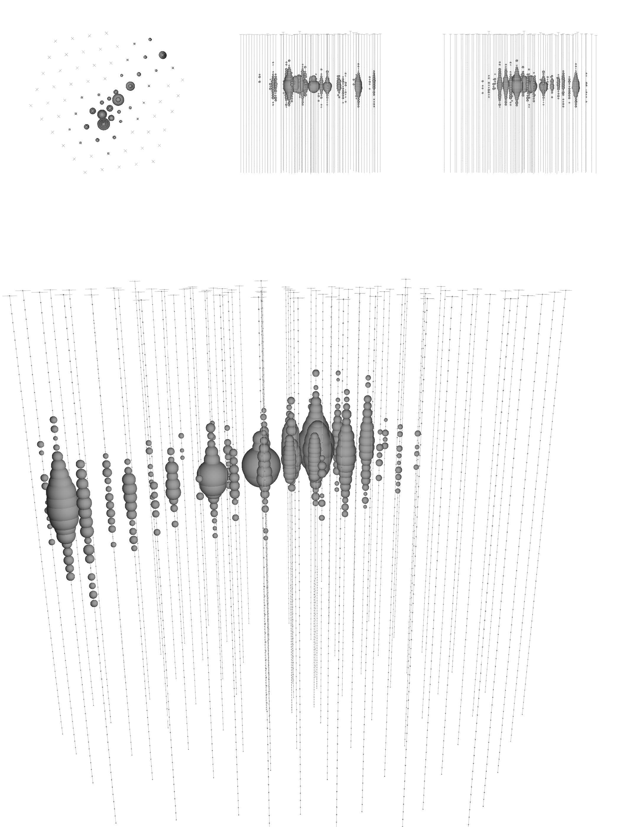
(a) A muon entering the detector and leaving only a small amount of energy behind.

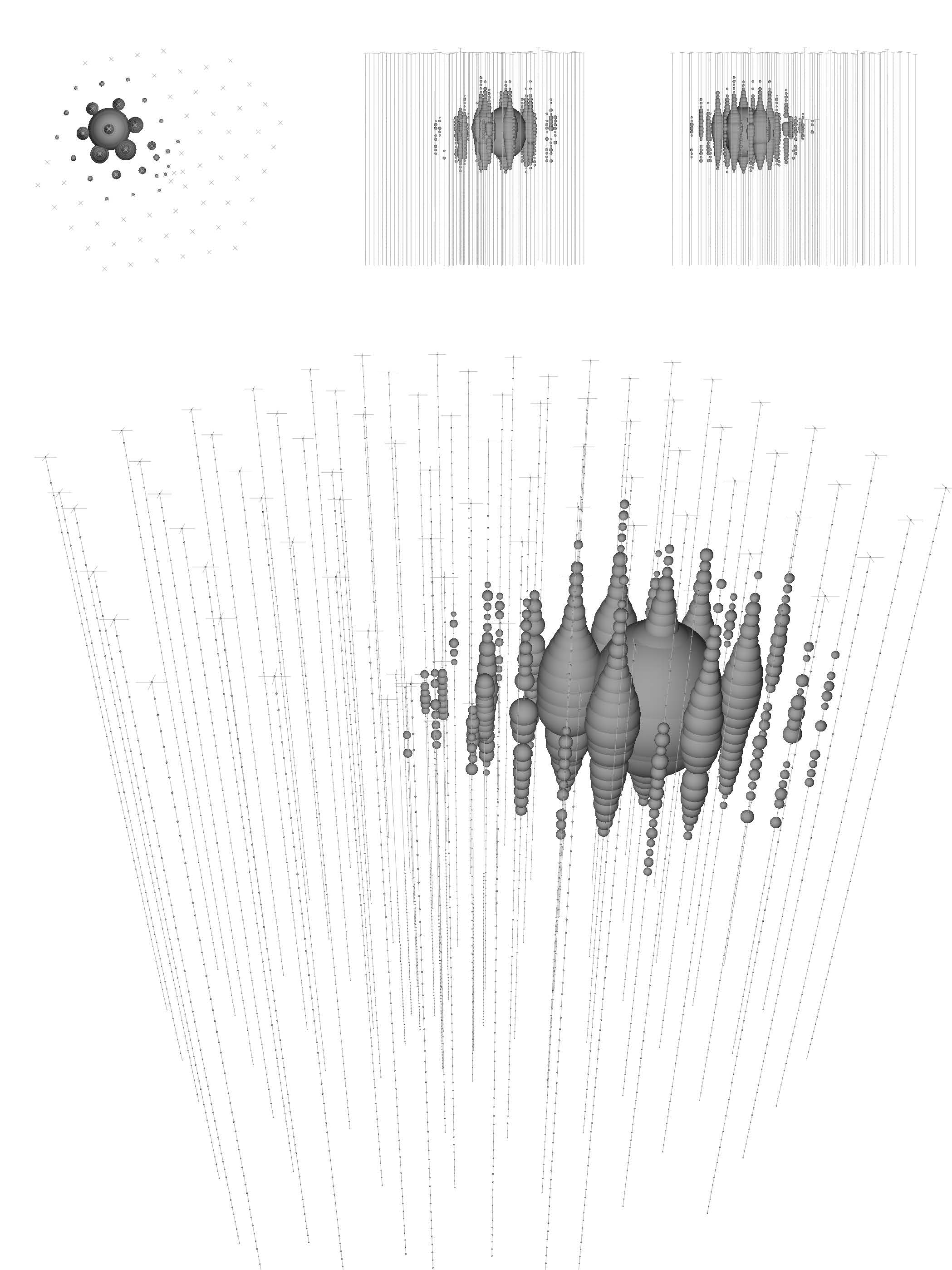
(b) A cascading burst event, with most of the energy remaining in the detector

Every measured event contains neutrinos, but there are some events where neutrinos are hard identify. In Figure 3, the left side shows muons escaping the detector, of which only a small amount of energy is left in the detector, while the right side shows a cascade of neutrino events, of which most of the energy is left in the detector. The right side represents perfect image, but impossible in reality because of the muon interference. For events that are difficult to reconstruct, we can focus on distinguishing atmospheric muons.

In the context of predicting atmospheric muons, a key strategy involves reconstructing their trajectories to understand whether the direction of muons was towards or away from the Earth. Given the inherent inability of muons to penetrate the Earth, “muons” travelling away from the Earth must be neutrinos. This technique allows to exclude noisy muons from analysis.

In addition, as shown in Figure 4, IceCube features zones with significant dust deposition, characterized by intense light absorption. Events occurring in these regions pose a considerable challenge for reconstruction and detection. [10]

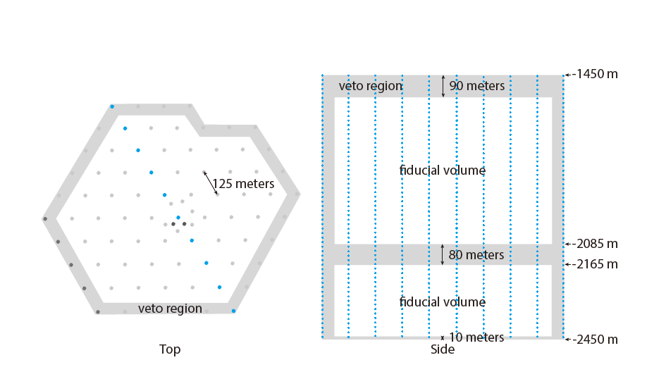
Figure4 Veto-Zone

After realizing this, we introduced the veto-zone. In the veto-region, we try to exclude muon and dust deposition regions, in order to obtain better quality pulse.

Then we applied this as filters for the event.

• Filter A. This filter involves event filtration based on angle and rejection zone criteria. The reconstruction difficulty of event is then computed, taking into account factors such as the horizontal direction, upward and downward considerations, veto-zone, and weights.
• Filter B. In this filter (also the original filter), events are discarded based on a time window. The effective time period is determined by considering the time when the pulse is at its strongest and the speed of light. The rank (or quality) of a pulse is subsequently calculated, considering the weight of the pulse size. The optimal pulse is selected based on these considerations.

Fitting – Apply the filters

Experiment 1

In this initial experiment, Filter A incorporates physical properties, while Filter B is a straightforward statistical filter. My initial assumption was that events filtered by Filter A would exhibit higher quality compared to Filter B. Consequently, I utilized Filter B data for pre-training and Filter A data for fine-tuning. Surprisingly, the results were discouraging and I thought about abandoning the approach.

Experiment 2

However, Experiment 2 completely changed the picture. Upon closer inspection, I realized that I had misapplied one of the model’s structures, leading to the omission of training for one of the models. Given the approaching end of the competition, retraining was impractical. Instead, I loaded a model initially trained on Filter A data and fine-tuned it using Filter B data — essentially reversing the sequence from Experiment 1.

Contrary to my expectations, this approach yielded very good results, surpassing my best cross-validation scores. This methodology was then applied across all models, propelling my solution into the top 3%.

After competition, I observed that some of the top solutions also employed a two-stage training approach. Notably, these models were trained on low and high pulses. In contrast, our solution leverages physical properties, delivering a new perspective on the task.

Final

IceCube competition definitely made me feel the fascination of science, like Prof. Francis Halzen said, ‘…what science is all about is not finding what you expect to find, is to find something you didn’t have any idea you were going to find, is to find the unexpected. '

Reference

[1] Ashley Chow, Lukas Heinrich, Philipp Eller, Rasmus Ørsøe, Sohier Dane. (2023). IceCube - Neutrinos in Deep Ice. Kaggle. https://kaggle.com/competitions/icecube-neutrinos-in-deep-ice

[2] Mirco Hunnefield Masters Thesis, Online Reconstruction of Muon-Neutrino Events in IceCube using Deep Learning Techniques

[3] Schatto, K. Stacked searches for high-energy neutrinos from blazars with IceCube. (Mainz U., 2014).

[4] R. Abbasi, M. Ackermann, J. Adams, et al., “Graph neural networks for low-energy event classification & reconstruction in icecube,” Journal of Instrumentation, vol. 17, no. 11, P11003, 2022.

[5] Schatto, Kai. Stacked searches for high-energy neutrinos from blazars with IceCube. Diss. Mainz, Univ., Diss., 2014, 2014.

[6] Lomax, Anthony, Alberto Michelini, and Dario Jozinović. “An investigation of rapid earthquake characterization using single‐station waveforms and a convolutional neural network.” Seismological Research Letters 90.2A (2019): 517-529.

[7] IceCube—Neutrinos in Deep Ice. (n.d.). Retrieved 25 January 2024, from https://kaggle.com/competitions/icecube-neutrinos-in-deep-ice

[8] Bukhari, Habib, et al. “IceCube–Neutrinos in Deep Ice The Top 3 Solutions from the Public Kaggle Competition.” arXiv preprint arXiv:2310.15674 (2023).

[9] Aartsen, Mark G., et al. “Energy reconstruction methods in the IceCube neutrino telescope.” Journal of Instrumentation 9.03 (2014): P03009.

[10] IceCube Collaboration*. “Evidence for high-energy extraterrestrial neutrinos at the IceCube detector.” Science 342.6161 (2013): 1242856.

[11] Aartsen, M. G. “Evidence for high-energy extraterrestrial neutrinos at the icecube detector. Science 342.” (2013).